shine's dev log
[Pytorch] Conditional GAN 구현 및 학습 (CGAN) 본문
1. 개요
https://github.com/godeastone/GAN-torch
Pytorch 로 구현한 CGAN 전체 코드는 위 git repository에서 확인할 수 있다.
2. Conditional GAN
Conditional GAN (CGAN)은 GAN이 처음 제안된 연도인 2014년 Mehdi Mirza, Simon Osindero 에 의해 제안된 GAN 의 변종 알고리즘이다.
아래 링크에서 논문 확인이 가능하다.
https://arxiv.org/abs/1411.1784
Conditional Generative Adversarial Nets
Generative Adversarial Nets [8] were recently introduced as a novel way to train generative models. In this work we introduce the conditional version of generative adversarial nets, which can be constructed by simply feeding the data, y, we wish to conditi
arxiv.org
Conditional GAN의 목적은 분명하다. Condition 이라는 조건을 나타내는 변수를 추가함으로써 데이터 생성을 '내 입맛대로' 할 수 있도록 한 것이다.
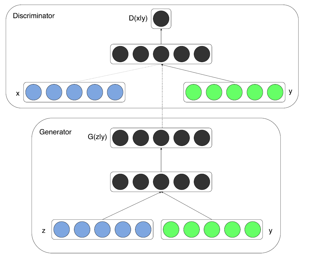
Conditional GAN은 [그림 1]과 같이 기존의 GAN 모델에서 단 하나, y 라는 condition 값이 추가되었다. 이 y 값은 Generator와 Discriminator의 Input값에 들어갈 때, 단순히 이어붙여주면 된다. (매우 간단)
예를 들어 MNIST 데이터셋을 GAN모델으로 학습하고 생성한다고 생각해보자.
어느정도 Generator 가 생성되었을 때, 하나의 데이터를 샘플링해보면 그 데이터 샘플은 분명 그럴듯한 숫자 모양을 하고 있을 것이다.
하지만, 그 숫자가 무슨 label에 해당하는 숫자인지는 까보기 전까지 구현한 사람도, 샘플링한 사람도 알지 못한다.
하지만 Condtional gan을 통해 이러한 문제를 해결할 수 있다.
학습 과정에서 숫자 0에 해당하는 데이터를 학습시킬때 latent 벡터 z 옆에 condition 변수 [1, 0, 0, 0, 0, 0, 0, 0, 0, 0] 를 이어붙여줘보자. (MNIST는 숫자이므로 총 10개의 label이 있고 이를 one-hot encoding 하여 벡터로 나타내주었다.)
또한, Generator를 통해 학습시킨 값 G(z)를 Discriminator에 넣어줄때도 동일하게 condition 변수 [1, 0, ..., 0] 을 이어붙여준채로 학습을 시켜보자.
마찬가지로 만약 2라는 데이터를 학습시킬때는 z 벡터와 G(z) 값 뒤에 condition 변수 [0, 0, 1, 0, 0, 0, 0, 0, 0, 0] 를 붙여주면 된다.
이렇게 학습시킬 경우, 나중에 학습 과정이 끝나고 샘플링 할때 G(z)에서 z 뒤에 자신이 원하는 label에 해당하는 condition 변수를 이어붙여준다면, 자신이 원하는 label에 해당하는 샘플을 얻어낼 수 있다.
즉 한마디로 정리해보면, GAN 학습과정에서 y라는 condition 변수를 추가함으로써 자신이 원하는 label의 데이터를 생산해낼 수 있도록 만든 GAN 모델. 이라고 보면 된다.
이렇게 단순해서인지 Conditional GAN의 loss 함수도 [그림 2] 에서 볼 수 있듯이 그냥 GAN 함수에 비해 단지 y 를 조건부 확률로 추가해준 것 밖에는 없다.

이외에도 논문을 보면, image 데이터를 CNN 연산하여 나온 fc layer를 condition으로 주고, 해당 사진을 설명하는 tag를 생성해낼 수 있는 모델도 확인해볼 수 있으니, 직접 논문을 읽어보는 것을 권장한다.
3. 구현
그럼 이제 CGAN을 어떻게 구현할 수 있을지 코드를 보며 이해해보자.
class Discriminator(nn.Module):
    def __init__(self):
        super(Discriminator, self).__init__()

        self.linear1 = nn.Linear(img_size + condition_size, hidden_size3)
        self.linear2 = nn.Linear(hidden_size3, hidden_size2)
        self.linear3 = nn.Linear(hidden_size2, hidden_size1)
        self.linear4 = nn.Linear(hidden_size1, 1)
        self.leaky_relu = nn.LeakyReLU(0.2)
        self.sigmoid = nn.Sigmoid()

    def forward(self, x):
        x = self.leaky_relu(self.linear1(x))
        x = self.leaky_relu(self.linear2(x))
        x = self.leaky_relu(self.linear3(x))
        x = self.linear4(x)
        x = self.sigmoid(x)
        return x
우선 Discriminator는 위와 같이 정의할 수 있다. 일반적인 multi layer neural network로 구성되어 있다.
총 4개의 Linear layer로 구성되어 있는데, 첫번째 layer에서는 MNIST 이미지 사이즈 (1 x 28 x 28 = 784)에 condition 변수의 크기 (condition_size)를 더한 값을 입력받고, 마지막 레이어에서는 classification을 위해 1개의 노드로 정리된다.
각 레이어 사이에는 activation function으로 leaky ReLU 함수가 사용되었으며, 마지막에는 확률로 표현하기 위해 sigmoid 함수가 사용되었다.
GAN과 다른점은 Input의 크기가 condition 변수의 크기만큼 더해졌다는 것밖에 없다.
class Generator(nn.Module):
    def __init__(self):
        super(Generator, self).__init__()

        self.linear1 = nn.Linear(noise_size + condition_size, hidden_size1)
        self.linear2 = nn.Linear(hidden_size1, hidden_size2)
        self.linear3 = nn.Linear(hidden_size2, hidden_size3)
        self.linear4 = nn.Linear(hidden_size3, img_size)
        self.relu = nn.ReLU()
        self.tanh = nn.Tanh()

    def forward(self, x):
        x = self.relu(self.linear1(x))
        x = self.relu(self.linear2(x))
        x = self.relu(self.linear3(x))
        x = self.linear4(x)
        x = self.tanh(x)
        return x
Generator는 Discriminator와 반대로 구성되어 있다.
역시 총 4개의 Linear layer로 구성되어 있으며, 입력값으로 noise vector 'z'의 크기에 condition 변수의 크기 (condition_size)를 더한 Input 값이 들어가고, 마지막 layer에서는 실제 MNIST 데이터의 크기 (1 x 28 x 28 = 784) 개의 노드로 정리된다.
각 layer 사이에는 activation function으로 ReLU 함수가 사용되었으며, 마지막 layer 에는 tanh 함수가 사용되었다.
Gnenrator 역시 GAN과 다른점은 Input의 크기가 condition 변수의 크기만큼 더해졌다는 것밖에 없다.
나머지 학습 과정은 GAN과 진짜 똑같다.
criterion = nn.BCELoss()
d_optimizer = torch.optim.Adam(discriminator.parameters(), lr=learning_rate)
g_optimizer = torch.optim.Adam(generator.parameters(), lr=learning_rate)
GAN과 마찬가지로 학습에는 BCELoss를 사용하였으며, Adam optimizer를 사용하였다.
GAN 에서도 강조했듯이, genrator와 discriminator는 서로 따로따로 학습되므로 각각 optimizer를 구분지어 정의해주어야 한다.
for epoch in range(num_epoch):
    for i, (images, label) in enumerate(data_loader):

        # 라벨을 만들어 줍니다. 1 for real, 0 for fake
        real_label =
        	torch.full((batch_size, 1), 1, dtype=torch.float32).to(device)
        fake_label =
        	torch.full((batch_size, 1), 0, dtype=torch.float32).to(device)

        # MNIST dataset의 데이터를 flatten 하게 reshape 해줍니다.
        real_images = images.reshape(batch_size, -1).to(device)
이제 for문을 통해 각 epoch 마다 학습을 시켜주게 된다.
학습을 위해 [batch size, 1] 크기의 모두 1로 구성된 real label 의 tensor와 모두 0으로 구성된 fake label의 tensor를 만들어 주었다.
	# +---------------------+
        # |   train Generator   |
        # +---------------------+

        # Initialize grad
        g_optimizer.zero_grad()
        d_optimizer.zero_grad()

        # fake image를 generator와 noize vector 'z' 를 통해 만들어주기
        z = torch.randn(batch_size, noise_size).to(device)

        # 노이즈 벡터 z 와 encoded labels을 합쳐준다. (concate)
        z_concat = torch.cat((z, label_encoded), 1)
        fake_images = generator(z_concat)
        fake_images_concat = torch.cat((fake_images, label_encoded), 1)

        # loss function에 fake image와 real label을 넘겨주기
        # 만약 generator가 discriminator를 속이면, g_loss가 줄어든다.
        g_loss = criterion(discriminator(fake_images_concat), real_label)

        # backpropagation를 통해 generator 학습
        g_loss.backward()
        g_optimizer.step()
우선 Generator를 학습시켜주자. Discriminator 를 먼저 학습시키든 Generator를 먼저 학습시키든 상관없지만, 중요한 것은 각자 따로따로 학습시켜줘야 한다는 점이다.
우선 noise vector 'z' 를 torch.randn 함수를 통해 랜덤한 값으로 채워준다.
[13번째 줄] 여기서 CGAN만의 특징이 나타나는데, 앞서 [그림 1]에서 보았던 구조처럼 noise vector 'z'에 label 값을 인코딩한 벡터(y) 를 합쳐줘야 한다.
[15번째 줄] 또한, Discriminator 의 Input에도 contion 변수가 합쳐져야 하므로, 생성된 fake image, G(z+y) 값에도 label 값을 인코딩한 벡터 (y)를 합쳐준다.
이제 앞서 선언한 generator에 (z+y) 를 넣어줌으로써 [28 x 28 = 784] 크기의 이미지 데이터를 생성하게 된다. 즉 G(z+y)는 Generator가 생성한 batch size 개수만큼의 이미지가 된다.
앞서 2장에서 설명했듯이 Generator는 D(G(z+y))의 성능을 낮추는 방향으로 학습된다.
따라서 loss 함수에 D(G(z+y))와 real label을 함께 넣어준다.
이렇게 할 경우, Discriminator가 제대로 판단을 할 경우(fake라 판단) Generator는 올바른 방향으로 데이터를 생성하지 못했다고 생각하게 되고, Discriminator 가 제대로 판단하지 못할 경우(real로 판단) Generator는 올바른 방향으로 데이터를 생성했다고 생각하게 된다.
이런 과정을 통해 Generator의 성능이 높아지는 방향으로 학습이 진행되게 된다.
        # +---------------------+
        # | train Discriminator |
        # +---------------------+

        # Initialize grad
        d_optimizer.zero_grad()
        g_optimizer.zero_grad()

        # fake image를 generator와 noize vector 'z' 를 통해 만들어주기
        z = torch.randn(batch_size, noise_size).to(device)

        # 노이즈 벡터 z 에 encoded label를 합쳐준다.
        z_concat = torch.cat((z, label_encoded), 1)
        fake_images = generator(z_concat)
        fake_images_concat = torch.cat((fake_images, label_encoded), 1)

        # fake image와 fake label, real image와 real label을 넘겨 loss 계산
        fake_loss = criterion(discriminator(fake_images_concat), fake_label)
        real_loss = criterion(discriminator(real_images_concat), real_label)
        d_loss = (fake_loss + real_loss) / 2

        # backpropagation을 통해 discriminator 학습
        # 이 부분에서는 generator는 학습시키지 않음
        d_loss.backward()
        d_optimizer.step()
다음으로 Discriminator를 학습시켜주자.
우선 앞서 했던것과 같이 (z+y) 값을 generator에 통과시켜 fake image를 만들어준다.
fake image에 역시 condition 변수 y를 합쳐 G(z+y) + y를 만들어준다.
D(G(z+y) + y) 값을 loss function에 fake label과 함께 넣어 fake loss를 구해주고, D(x) 값을 loss function에 real label과 함게 넣어 real loss를 구해준다.
이렇게 구한 두 fake / real loss를 평균내서 전체 discriminator 의 loss값을 구해준다.
이렇게 하면 Discriminator가 제대로 fake 와 real 이미지를 판단할 수 있는 방향으로 학습이 진행되게 된다.
이제 conditional GAN의 꽃이라 불릴 수 있는 '내가 원하는 label의 데이터를 샘플링' 하는 것을 해보자.
# CGAN's 의 validity를 테스트해볼 수 있는 함수
def check_condition(_generator):
    test_image = torch.empty(0).to(device)

    for i in range(10):
        test_label = torch.tensor([0, 1, 2, 3, 4, 5, 6, 7, 8, 9])
        test_label_encoded = F.one_hot(test_label, num_classes=10).to(device)

        # create noise(latent vector) 'z'
        _z = torch.randn(10, noise_size).to(device)
        _z_concat = torch.cat((_z, test_label_encoded), 1)

        test_image = torch.cat((test_image, _generator(_z_concat)), 0)

    _result = test_image.reshape(100, 1, 28, 28)
    save_image(_result, os.path.join(dir_name, 'CGAN_test_result.png'), nrow=10)
CGAN이 제대로 동작하는지는 check_condition 이라는 함수를 통해 구현했다.
학습된 generator를 parameter로 받아온 check_condition 함수는 test_label_encoded라는 [10 x 10]의 matrix를 만들어낸다.
test_label_encoded 는 각 열마다 0, 1, 2, ..., 9에 해당하는 encoded vector가 담겨있다. 한번 나타내보면 아래와 같다.
[1, 0, 0, 0, 0, 0, 0, 0, 0, 0]
[0, 1, 0, 0, 0, 0, 0, 0, 0, 0]
[0, 0, 1, 0, 0, 0, 0, 0, 0, 0]
[0, 0, 0, 1, 0, 0, 0, 0, 0, 0]
. . .
[0, 0, 0, 0, 0, 0, 0, 0, 1, 0]
[0, 0, 0, 0, 0, 0, 0, 0, 0, 1]
이제 noise vector 'z' 10행을 만들어내고, 거기에 test_label_encoded matrix를 이어준 _z_concat 값을 만들어준다. 이어붙이면 [10 x 20] 의 크기가될 것이다.
generator에 _z_concat을 넣어주면, 샘플링한 이미지가 나타나게 될 것이다.
차례로 0, 1, 2, ..., 9에 해당하는 label vector를 붙여줬으므로, 실제 샘플링한 값도 이에 맞게 나올 것이다.
실제 코드를 돌려 GAN을 학습한 뒤, check_condition을 통해 확인한 결과는 [그림 3]과 같다.

실제로 내가 원하는 condition대로 잘 학습된 것을 확인할 수 있다. (대체로 2랑 5를 조금 잘 못만들어내는 듯,,)
만약 기본 GAN을 통해 학습시켰다면, [그림 3]에 무작위의 숫자들이 들어갔을 것이다.
위 내용은 공부하며 정리한 것으로, 오류가 있을 수 있습니다.
'머신러닝' 카테고리의 다른 글
| [Pytorch] GAN 구현 및 학습 (2) | 2022.03.12 |
|---|---|
| [ML] Deepfake Detection 성능 분석 (8) | 2022.02.26 |
| KL divergence와 JSD의 개념 (feat. cross entropy) (1) | 2022.02.19 |
| [Recommender system] 영화 추천 시스템 (0) | 2022.01.23 |
| PCA (Principal Component Analysis) : 주성분 분석 이란? (36) | 2021.12.21 |


